VectorPostProcessing package

Submodules

VectorPostProcessing.animate_var_vector_setup module

Temporal Animation of MESH Variables from Vector and NetCDF Data

This module generates animated GIFs of spatially-distributed MESH model outputs (e.g., Discharge, Snow, Precipitation) over time using shapefiles and corresponding NetCDF files. It supports daily, monthly, and yearly animations.

The function processes time-aware variables stored in NetCDF files and overlays them on subbasin polygons, producing frame-by-frame maps and exporting the animation as a .gif file using Matplotlib and Pillow.

Function: animate_mesh_outputs_to_gif

Description:

Generates animated visualizations for MESH model state or flux variables across subbasins, overlaying spatial values on a shapefile with optional layer suffixes and colorbars. Output is saved as an animated .gif.

Parameters:

• shapefile_pathstr

  Path to the subbasin shapefile (must include a COMID field).

• netcdf_dirstr

  Directory containing NetCDF variable files (e.g., QO_M_GRD.nc, SNO_M_GRD.nc).

• ddb_pathstr

  Path to the MESH drainage database NetCDF file used to extract subbasin IDs.

• varnameslist of str

  List of variable names to animate (e.g., [‘QO’, ‘SNO’, ‘PREC’]).

• filenameslist of str

  List of NetCDF filenames corresponding to each variable (same order as varnames).

• cbar_labelslist of str

  List of colorbar labels for each variable (e.g., [‘Discharge [m³/s]’, ‘Snow Mass [mm]’, ‘Precipitation [mm]’]).

• outdirstr

  Output directory to save the generated .gif files.

• modestr, optional (default=’monthly’)

  Time mode for animation. Options: ‘daily’, ‘monthly’, or ‘yearly’.

• domain_namestr, optional (default=’Basin’)

  Prefix to use in animated titles and output filenames.

• cmapstr, optional (default=’gnuplot2_r’)

  Matplotlib colormap to use for the animation.

• subbasin_varstr, optional

  Name of the subbasin variable in the NetCDF drainage database (default: ‘subbasin’).

Input Format:

1. Subbasin shapefile (.shp) with a COMID field

2. Drainage database (.nc) with subbasin variable

3. NetCDF model output files with time and subbasin dimensions

Output:

• .gif animations for each variable saved in outdir

• Each frame shows spatial distribution for a time step

• Colorbars, labels, and layer info auto-handled

Example Usage:

>>> from VectorPostProcessing.animate_var_vector_setup import animate_mesh_outputs_to_gif

>>> animate_mesh_outputs_to_gif(
...     shapefile_path='D:/HydrologicalModels/MESH/Baseline/sras-agg-model_1/sras_MESH_PostProcessing/GIS/sras_subbasins_MAF_Agg.shp',
...     netcdf_dir='D:/HydrologicalModels/MESH/Baseline/sras-agg-model_1/sras_MESH_PostProcessing/BASINAVG4',
...     ddb_path='D:/HydrologicalModels/MESH/Baseline/sras-agg-model_1/MESH-sras-agg/MESH_drainage_database.nc',
...     varnames=['QO', 'SNO', 'PREC'],
...     filenames=['QO_Y_GRD.nc', 'SNO_Y_GRD.nc', 'PREC_Y_GRD.nc'],
...     cbar_labels=['Discharge [m³/s]', 'Snow Mass [mm]', 'Precipitation [mm]'],
...     outdir='D:/Coding/GitHub/Repos/MESH-Scripts-PyLib/VectorPostProcessing/ExampleFiles/Outputs',
...     mode='Yearly',
...     domain_name='SrAs',
...     subbasin_var='subbasin'
... )

>>> # This will create animated GIFs for each variable in the specified output directory.
>>> # The GIFs will be named as follows:

>>> # QO_yearly_animation.gif
>>> # SNO_yearly_animation.gif
>>> # PREC_yearly_animation.gif

Dependencies:

• geopandas

• matplotlib

• netCDF4

• pandas

• numpy

• xarray

• Pillow (via matplotlib.animation.PillowWriter)

VectorPostProcessing.animate_var_vector_setup.animate_mesh_outputs_to_gif(shapefile_path, netcdf_dir, ddb_path, varnames, filenames, cbar_labels, outdir, mode='monthly', domain_name='Basin', cmap='gnuplot2_r', comid_field='COMID', subbasin_var='subbasin')

VectorPostProcessing.plt_var_vector_setup module

Spatial Variable Visualization from Vector and NetCDF Files

This module provides a unified plotting interface to visualize spatial variables from NetCDF datasets (e.g., MESH drainage database or parameters file) overlaid on a vector shapefile (e.g., subbasin polygons). It supports: - Single variable plotting per subbasin - Multi-class land use variable visualization (e.g., GRUs) - Layer-wise soil variable visualization (e.g., SAND, CLAY, OC)

It automatically interprets the variable’s dimensions to choose the appropriate visualization layout (single map or subplots).

Function: plt_var_from_vector_ddb_netcdf

Description:

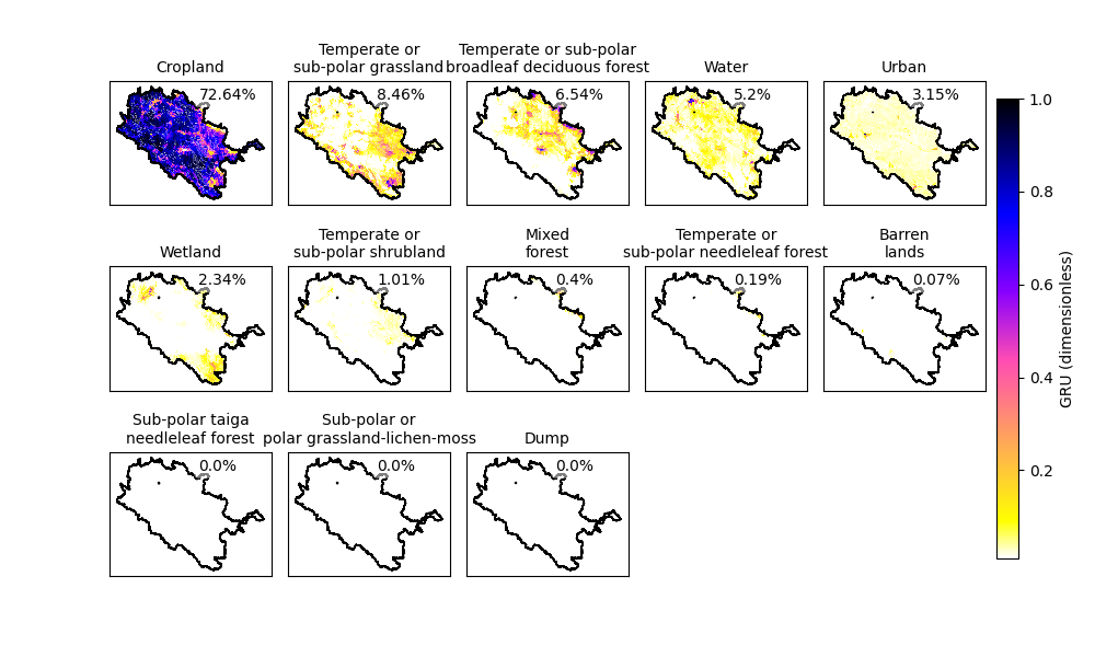
Plots spatial variables stored in NetCDF files on top of vector shapefiles using GeoPandas and Matplotlib. This function is useful for visualizing hydrological model inputs such as Grouped Respone Units (GRUs), soil layers (e.g., SAND, CLAY), or other scalar variables (e.g., Elevation, Drainage Area) in spatial context.

Parameters:

• output_basin_pathstr

  Full path to the basin shapefile (.shp). Must contain a unique subbasin identifier column (e.g., ‘COMID’).

• ddbnetcdf_pathstr

  Path to the input NetCDF file containing the spatial variable (e.g., MESH_drainage_database.nc or MESH_parameters.nc).

• variable_namestr

  Name of the variable to extract and visualize from the NetCDF file.

• save_pathstr, optional (default=’plot.png’)

  Full path to save the output image file (.png).

• text_locationtuple, optional (default=(0.55, 0.95))

  (x, y) coordinates in axes fraction (0–1) to place text annotations inside each subplot.

• font_sizeint, optional (default=10)

  Font size for subplot titles and annotations.

• cmapstr, optional (default=’viridis’)

  Matplotlib colormap to use for shading data values.

• cbar_locationlist of float, optional (default=[0.96, 0.15, 0.02, 0.7])

  Location of colorbar [left, bottom, width, height] in normalized figure coordinates.

• subplot_adjustmentsdict, optional

  Dictionary of subplot spacing and padding adjustments passed to fig.subplots_adjust(). Example: {‘left’: 0.1, ‘right’: 0.9, ‘bottom’: 0.1, ‘top’: 0.9, ‘wspace’: 0.1, ‘hspace’: 0.2}

• subbasin_varstr, optional (default=’subbasin’)

  Name of the NetCDF variable that contains subbasin indices.

• comid_varstr, optional (default=’COMID’)

  Name of the shapefile column used to join NetCDF data to the shapefile geometry.

• landuse_classeslist of str, optional

  Used when variable_name has GRU land use classes. Overrides land use names from the NetCDF file.

• grudimstr, optional (default=’NGRU’)

  Name of the NetCDF dimension for land use classes.

• grunames_varstr, optional (default=’LandUse’)

  Name of the NetCDF variable containing land use class names.

• soldimstr, optional (default=’nsol’)

  Name of the NetCDF dimension representing soil layers.

• vminfloat, optional

  Lower bound for color scaling. If not provided, determined automatically per variable type.

• vmaxfloat, optional

  Upper bound for color scaling. If not provided, determined automatically per variable type.

• sort_gru_by_meanbool, optional (default=True)

  If True, sorts GRUs by mean area fraction and adds percentage annotations in each subplot. If False, plots GRUs in original order with no annotation.

Processing Logic:

• If variable_name has 1D dimension (e.g., [subbasin]), a single map is plotted.

• If it has 2D shape with land use dim (e.g., [subbasin, NGRU]), a grid of subplots is created per GRU.

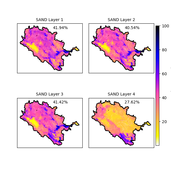
• If it has 2D shape with soil layer dim (e.g., [subbasin, nsol]), a grid of subplots is created per soil layer.

Input Format:

1. Shapefile (.shp) with a subbasin identifier column (e.g., ‘COMID’)

2. NetCDF file (.nc) with variables such as: - lat, lon - 1D or 2D variable of interest (e.g., GRU, SAND) - Dimension definitions for subbasin, land use, or soil layers

Output:

• A static plot (.png) saved at save_path location

• Subplots with dissolved basin outline and percentage annotations

• Shared colorbar with variable name and units

Example Usage:

>>> import os
>>> from VectorPostProcessing.plt_var_vector_setup import plt_var_from_vector_ddb_netcdf

>>> # Example 1: GRU (Grouped Land Use Classes) Visualization
>>> base_dir = 'D:/Coding/GitHub/Repos/MESH-Scripts-PyLib/VectorPostProcessing/ExampleFiles'
>>> shapefile_path = os.path.join(base_dir, 'sras_subbasins_MAF_Agg.shp')
>>> netcdf_path = os.path.join(base_dir, 'MESH_drainage_database.nc')
>>> output_path = os.path.join(base_dir, 'Outputs', 'GRU.png')
>>> lclass = [
...     'Temperate or sub-polar needleleaf forest', 'Sub-polar taiga needleleaf forest',
...     'Temperate or sub-polar broadleaf deciduous forest', 'Mixed forest',
...     'Temperate or sub-polar shrubland', 'Temperate or sub-polar grassland',
...     'Sub-polar or polar grassland-lichen-moss', 'Wetland', 'Cropland',
...     'Barren lands', 'Urban', 'Water', 'Dump'
... ]
>>> plt_var_from_vector_ddb_netcdf(
...     output_basin_path=shapefile_path,
...     ddbnetcdf_path=netcdf_path,
...     variable_name='GRU',
...     save_path=output_path,
...     text_location=(0.55, 0.95),
...     font_size=10,
...     cmap='gnuplot2_r',
...     cbar_location=[0.91, 0.15, 0.02, 0.7],
...     subplot_adjustments={'left': 0.1, 'right': 0.9, 'bottom': 0.1, 'top': 0.9, 'wspace': 0.1, 'hspace': 0.2},
...     subbasin_var='subbasin',
...     comid_var='COMID',
...     landuse_classes=lclass,
...     grudim='NGRU',
...     grunames_var='LandUse',
        soldim='nsol',    # from netcdf parameter file
        vmin=None,
    sort_gru_by_mean: bool = True,
        vmax=None
... )

>>> # Example 2: Soil Variable Visualization (e.g., SAND across layers)
>>> netcdf_path = os.path.join(base_dir, 'MESH_parameters.nc')
>>> output_path = os.path.join(base_dir, 'Outputs', 'SAND.png')
>>> plt_var_from_vector_ddb_netcdf(
...     output_basin_path=shapefile_path,
...     ddbnetcdf_path=netcdf_path,
...     variable_name='SAND',
...     save_path=output_path,
...     text_location=(0.55, 0.95),
...     font_size=10,
...     cmap='gnuplot2_r',
...     cbar_location=[0.91, 0.15, 0.02, 0.7],
...     subplot_adjustments={'left': 0.1, 'right': 0.9, 'bottom': 0.1, 'top': 0.9, 'wspace': 0.1, 'hspace': 0.2},
...     subbasin_var='subbasin',
...     comid_var='COMID'
... )

Notes:

• All spatial plotting is done in EPSG:4326 (WGS84)

• The function automatically merges the NetCDF data with shapefile geometry using the specified ID fields

• Color scaling (vmin, vmax) and transparency for 0 values is handled internally

Dependencies:

• geopandas

• pandas

• matplotlib

• numpy

• netCDF4

VectorPostProcessing.plt_var_vector_setup.plt_var_from_vector_ddb_netcdf(output_basin_path, ddbnetcdf_path, variable_name, save_path='plot.png', text_location=(0.55, 0.95), font_size=10, cmap='viridis', cbar_location=[0.96, 0.15, 0.02, 0.7], subplot_adjustments=None, subbasin_var='subbasin', comid_var='COMID', landuse_classes=None, grudim='NGRU', grunames_var='LandUse', soldim='nsol', vmin=None, sort_gru_by_mean: bool = True, vmax=None)

VectorPostProcessing.save_mesh_outputs_as_png module

VectorPostProcessing.save_mesh_outputs_as_png.save_mesh_outputs_as_png(shapefile_path, netcdf_dir, ddb_path, varnames, filenames, cbar_labels, outdir, indices_to_save, mode='monthly', domain_name='Basin', cmap='gnuplot2_r', comid_field='COMID', subbasin_var='subbasin')

Generate and save static PNG plots of MESH model output variables for specific time slices.

This function overlays MESH model output (e.g., discharge, snow, temperature) from NetCDF files onto a shapefile representing subbasin polygons. For each variable and selected time index, a PNG figure is generated with consistent colorbar scales and custom titles based on domain, variable, and time.

Parameters:

• shapefile_path (str) – Path to the shapefile (.shp) representing the subbasins with a ‘COMID’ field.

• netcdf_dir (str) – Directory containing the NetCDF output files.

• ddb_path (str) – Path to the NetCDF drainage database containing the ‘subbasin’ variable used for merging.

• varnames (list of str) – List of variable names to extract from each NetCDF file (e.g., [‘QO’, ‘SNO’]).

• filenames (list of str) – List of NetCDF filenames corresponding to each variable in varnames.

• cbar_labels (list of str) – List of labels for the colorbars corresponding to each variable.

• outdir (str) – Directory where output PNG figures will be saved.

• indices_to_save (list of int) – List of time indices to extract and plot (e.g., [0, 1, 5]).

• mode ({'daily', 'monthly', 'yearly', 'hourly'}, optional) – Time resolution of the data for labeling the figures. Default is ‘monthly’.

• domain_name (str, optional) – Name of the domain used in the figure title. Default is ‘Basin’.

• cmap (str, optional) – Matplotlib colormap to use for the plots. Default is ‘gnuplot2_r’.

• subbasin_var (str, optional) – Name of the subbasin variable in the NetCDF drainage database (default: ‘subbasin’).

Returns:

Saves PNG image files to the specified output directory.

Return type:

None

Raises:

ValueError – If an unsupported mode is provided for the mode parameter.

Notes

• Assumes that each NetCDF file contains a ‘time’ dimension and that values begin from index 1 (skipping index 0).

• Automatically adjusts date labeling based on the selected time mode.

• Supports automatic detection of layer (e.g., ‘Layer1’, ‘Layer2’) from filenames using ‘IG1’, ‘IG2’, etc.

Example

>>> save_mesh_outputs_as_png(
...     shapefile_path='shapes/sras_subbasins.shp',
...     netcdf_dir='outputs/monthly',
...     ddb_path='outputs/MESH_drainage_database.nc',
...     varnames=['QO', 'SNO'],
...     filenames=['QO_Y_GRD.nc', 'SNO_Y_GRD.nc'],
...     cbar_labels=['Discharge [m³/s]', 'Snow [mm]'],
...     outdir='outputs/pngs',
...     indices_to_save=[0, 3, 6],
...     mode='monthly',
...     domain_name='SrAs',
...     cmap='viridis',
...     subbasin_var='subbasin'
... )

Module contents